Introduction
Understanding and predicting customer behavior is crucial for business success. This case study explores how a specialty coffee company leveraged decision trees and random forests to gain insights into their customer base and make informed business decisions.
Our challenge: predict whether customers would purchase a new product - Hidden Farm coffee - based on demographic and purchasing variables. This type of prediction is common across industries and can inform various business strategies, including:
- Product development
- Marketing strategy
- Inventory management
- Customer retention efforts
The Dataset
We used a publicly available dataset from this GitHub repository. It contains customer information and purchase history for our hypothetical coffee company, including:
- Customer age
- Gender
- Salary
- Online purchase history
- Distance from the flagship store
- Recent spending on coffee products
- Number of coffee bean shipments ordered in the past year
Data Exploration and Visualization
After cleaning our dataset, we performed exploratory data analysis (EDA) to gain insights into our customer base and their purchasing behaviors.
Boxplot Analysis: Spending vs. Purchase Decision
We started by comparing weekly spending between customers who made a purchase and those who didn’t.
plt.figure(figsize=(8, 6))
sns.boxplot(data=NoPrediction, x='Decision', y='spent_last_week')
plt.title('Boxplot of Decision vs. spent_last_week')
plt.xlabel('Decision')
plt.ylabel('spent_last_week')
plt.show()
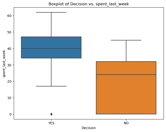
While this boxplot suggests that customers who have bought at least one RR Diner Coffee product online tend to spend more in the last week than those who haven’t, we can’t draw definitive conclusions without statistical testing.
Scatterplot Analysis: Distance, Monthly Spending, and Purchase Decision
Next, we explored the relationship between a customer’s distance from the flagship store, their monthly spending, and their purchase decision.
plt.figure(figsize=(10, 6))
sns.scatterplot(data=NoPrediction, x='Distance', y='spent_last_month', hue='Decision')
plt.title('Scatterplot of distance vs. spent_last_month (colored by Decision)')
plt.xlabel('Distance')
plt.ylabel('Spent Last Month')
plt.legend(title='Decision')
plt.show()
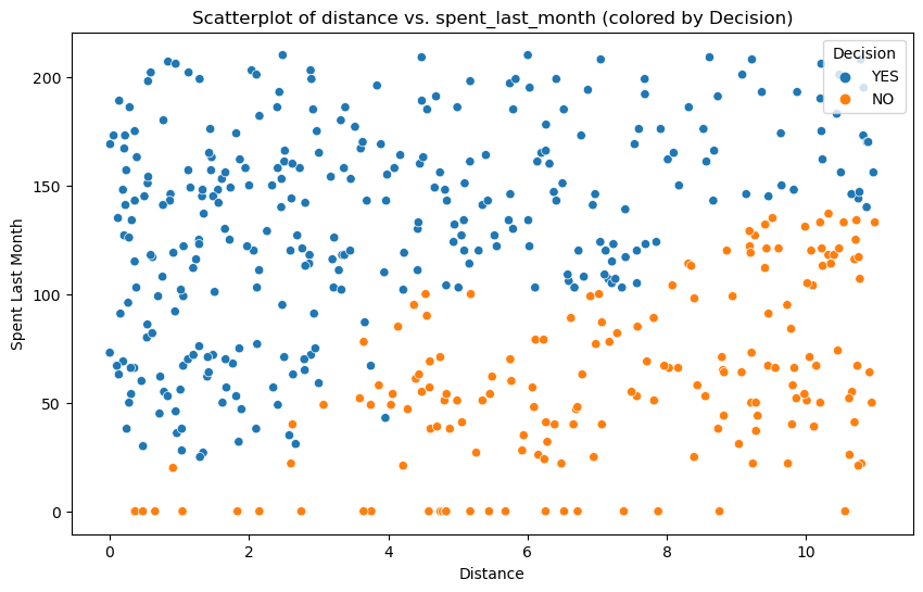
Interestingly, for customers who have purchased online, proximity to a flagship store seems to correlate positively with monthly spending. Conversely, for those who haven’t purchased online, spending increases with distance from the flagship store.
Choosing a Modeling Approach
Our exploratory data analysis revealed complex relationships between variables and potential non-linear patterns in customer behavior. To capture these intricacies and create a predictive model that’s both accurate and interpretable, we needed a versatile and robust approach. This led us to consider decision trees as our primary modeling technique.
Why Decision Trees?
We chose decision trees as our primary method for this analysis due to several key advantages:
- Interpretability: Decision trees provide a clear, visual representation of the decision-making process.
- Handling Mixed Data Types: They can work with both categorical and numerical data without extensive preprocessing.
- Capturing Non-linear Relationships: Unlike linear models, decision trees can capture complex, non-linear relationships between variables.
- Feature Importance: They inherently provide information about which features are most important for prediction.
These characteristics make decision trees particularly well-suited for our task of predicting customer purchases while providing actionable insights for our business strategy.
Modeling
We created four different decision tree models to predict whether customers would buy the product:
- Entropy model with no maximum depth
- Gini impurity model with no maximum depth
- Entropy model with maximum depth of 3
- Gini impurity model with maximum depth of 3
Model 1: Entropy model - No Max Depth
# Create and train the model
model_1 = tree.DecisionTreeClassifier(criterion='entropy', random_state=42)
model_1.fit(X_train, y_train)

# Make predictions
y_pred_1 = model_1.predict(X_test)

# Visualize the tree
exported = tree.export_graphviz(model_1,
                           out_file=None,
                           feature_names=X_train.columns,
                           class_names=['No', 'Yes'],
                           filled=True,
                           rounded=True,
                           special_characters=True)

graph = graphviz.Source(exported)
graph.format = 'png'
graph.render('decision_tree_entropy_model')
Image(filename='decision_tree_entropy_model.png')

# Evaluate the model
print("Model Entropy - no max depth")
print("Accuracy:", metrics.accuracy_score(y_test, y_pred_1))
print("Balanced accuracy:", metrics.balanced_accuracy_score(y_test, y_pred_1))
print('Precision score for "Yes"', metrics.precision_score(y_test, y_pred_1, pos_label="YES"))
print('Precision score for "No"', metrics.precision_score(y_test, y_pred_1, pos_label="NO"))
print('Recall score for "Yes"', metrics.recall_score(y_test, y_pred_1, pos_label="YES"))
print('Recall score for "No"', metrics.recall_score(y_test, y_pred_1, pos_label="NO"))
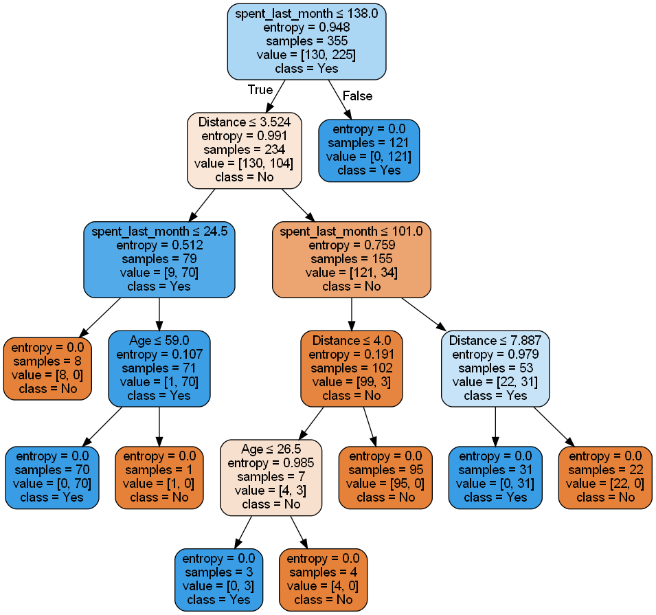
This model uses entropy as the criterion for splitting nodes and doesn’t set a maximum depth for the tree. Entropy measures the impurity or uncertainty in the dataset. The model is trained on the training data and then used to make predictions on the test data.
We visualize the tree using the export_graphviz function from scikit-learn, which allows us to create a graphical representation of the decision tree. This visualization helps in understanding the structure and decision-making process of the model.
The model’s performance is evaluated using several metrics:
- Accuracy: 0.9916 (99.16% of predictions are correct)
- Balanced accuracy: 0.9878 (accounts for imbalanced classes)
- Precision for “Yes”: 0.9873 (98.73% of positive predictions are correct)
- Precision for “No”: 1.0000 (100% of negative predictions are correct)
- Recall for “Yes”: 1.0000 (100% of actual positive cases are correctly identified)
- Recall for “No”: 0.9756 (97.56% of actual negative cases are correctly identified)
These metrics indicate that the model performs exceptionally well, with high accuracy, precision, and recall for both classes. The perfect recall for “Yes” suggests that the model doesn’t miss any positive cases, while the slightly lower recall for “No” indicates that it misclassifies a small number of negative cases as positive.
The high performance across all metrics suggests that this model is very effective at predicting customer behavior based on the given features. However, it’s important to consider that such high performance might indicate potential overfitting, especially since there’s no depth limit on the tree. Comparing this model’s performance with the other models, especially those with depth constraints, will help in assessing its generalizability.
Model 2: Gini impurity model - No Max Depth
# Create and train the model
model_2 = tree.DecisionTreeClassifier(criterion='gini', random_state=246)
model_2.fit(X_train, y_train)

# Make predictions
y_pred_2 = model_2.predict(X_test)

# Visualize the tree
exported = tree.export_graphviz(model_2,
                           out_file=None,
                           feature_names=X_train.columns,
                           class_names=model_2.classes_,
                           filled=True,
                           rounded=True,
                           special_characters=True)

graph = graphviz.Source(exported)
graph.format = 'png'
graph.render('decision_tree_gini_model')
Image(filename='decision_tree_gini_model.png')

# Evaluate the model
print("Model Gini impurity model")
print("Accuracy:", metrics.accuracy_score(y_test, y_pred_2))
print("Balanced accuracy:", metrics.balanced_accuracy_score(y_test, y_pred_2))
print('Precision score', metrics.precision_score(y_test, y_pred_2, pos_label="YES"))
print('Recall score', metrics.recall_score(y_test, y_pred_2, pos_label="NO"))
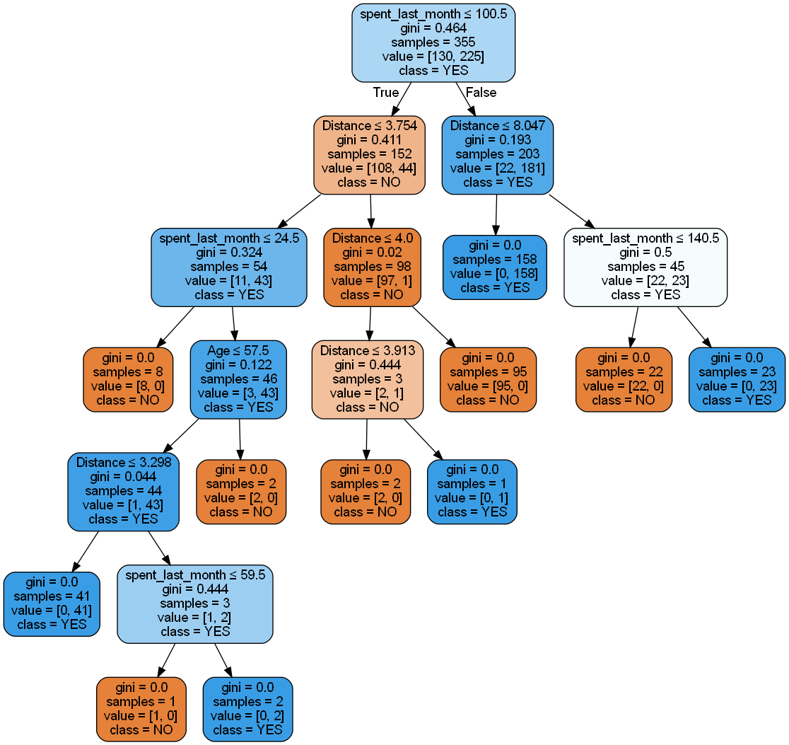
This model uses Gini impurity as the criterion for splitting nodes and, like Model 1, doesn’t set a maximum depth for the tree. Gini impurity is another measure of the quality of a split, similar to entropy but computationally simpler as it doesn’t require logarithmic calculations.
The model’s performance metrics are:
- Accuracy: 0.9832 (98.32% of predictions are correct)
- Balanced accuracy: 0.9814 (accounts for imbalanced classes)
- Precision for “Yes”: 0.9872 (98.72% of positive predictions are correct)
- Recall for “No”: 0.9756 (97.56% of actual negative cases are correctly identified)
Comparison with Model 1 (Entropy):
- Accuracy: The Gini model (98.32%) is slightly less accurate than the Entropy model (99.16%).
- Balanced accuracy: The Gini model (98.14%) performs slightly worse than the Entropy model (98.78%).
- Precision for “Yes”: The Gini model (98.72%) is marginally lower than the Entropy model (98.73%).
- Recall for “No”: Both models have the same recall for “No” (97.56%).
Overall, the Entropy model (Model 1) slightly outperforms the Gini model (Model 2), but the differences are minor. Both models show excellent performance, with accuracy and other metrics above 98%. The choice between these models might come down to computational efficiency in larger datasets, where Gini’s simpler calculations could provide a speed advantage.
As with Model 1, the high performance of Model 2 suggests that it’s very effective at predicting customer behavior based on the given features. However, the lack of depth limitation in both models could potentially lead to overfitting. Further evaluation, such as cross-validation or testing on a separate dataset, would be beneficial to assess the models' generalization capabilities.
Model 3: Entropy model - Max Depth 3
# Create and train the model
model_3 = tree.DecisionTreeClassifier(criterion='entropy', max_depth=3, random_state=246)
model_3.fit(X_train, y_train)

# Make predictions
y_pred_3 = model_3.predict(X_test)

# Visualize the tree
exported = tree.export_graphviz(model_3,
                                out_file=None,
                                feature_names=X_train.columns,
                                class_names=model_3.classes_,
                                filled=True,
                                rounded=True,
                                special_characters=True)

graph = graphviz.Source(exported)
graph.format = 'png'
graph.render('decision_tree_entropy_model_depth_3')
Image(filename='decision_tree_entropy_model_depth_3.png')

# Evaluate the model
print("Model Entropy model max depth 3")
print("Accuracy:", metrics.accuracy_score(y_test, y_pred_3))
print("Balanced accuracy:", metrics.balanced_accuracy_score(y_test, y_pred_3))
print('Precision score for "Yes"', metrics.precision_score(y_test, y_pred_3, pos_label="YES"))
print('Recall score for "No"', metrics.recall_score(y_test, y_pred_3, pos_label="NO"))
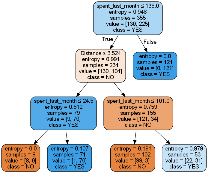
This model uses entropy as the criterion for splitting nodes, like Model 1, but introduces a maximum depth constraint of 3 levels. This constraint aims to prevent overfitting by limiting the complexity of the tree.
The model’s performance metrics are:
- Accuracy: 0.9832 (98.32% of predictions are correct)
- Balanced accuracy: 0.9814 (accounts for imbalanced classes)
- Precision for “Yes”: 0.9872 (98.72% of positive predictions are correct)
- Recall for “No”: 0.9756 (97.56% of actual negative cases are correctly identified)
Comparison with Model 1 (Entropy, no max depth):
- Accuracy: Slightly lower (98.32% vs 99.16%)
- Balanced accuracy: Slightly lower (98.14% vs 98.78%)
- Precision for “Yes”: Slightly lower (98.72% vs 98.73%)
- Recall for “No”: Same (97.56%)
Despite the depth limitation, Model 3 maintains excellent performance, with only a slight decrease in accuracy and other metrics compared to the unrestricted Model 1. This constrained model offers significant advantages in terms of simplicity and interpretability. The max depth of 3 results in a much simpler tree structure, which is easier to understand and explain – a valuable asset in business contexts where model interpretability is crucial. While the unrestricted Model 1 showed slightly better performance on the test set, it may be more prone to overfitting. Model 3’s simpler structure might generalize better to new, unseen data. With a max depth of 3, we can clearly identify which features the model considers most important for classification, providing valuable insights into the key factors influencing customer behavior. Additionally, a shallower tree is computationally more efficient, which can be beneficial when dealing with larger datasets or when prediction speed is important. In conclusion, while Model 3 shows a slight decrease in performance metrics compared to Model 1, the trade-off is minimal. The constrained model’s advantages in simplicity, interpretability, and potential for better generalization suggest that it might be preferable in many practical applications, especially when model explainability is a priority. This balance between performance and interpretability makes Model 3 a strong candidate for real-world deployment in customer behavior prediction scenarios.
Model 4: Gini impurity model - max depth 3
# Create and train the model
gini_model2 = tree.DecisionTreeClassifier(criterion='gini', random_state=246, max_depth=3)
gini_model2.fit(X_train, y_train)

# Make predictions
y_pred2 = gini_model2.predict(X_test)

# Visualize the tree
dot_data = StringIO()
tree.export_graphviz(gini_model2, out_file=dot_data,
                feature_names=X_train.columns,
                class_names=gini_model2.classes_.astype(str),
                filled=True, rounded=True,
                special_characters=True)

graph = graphviz.Source(dot_data.getvalue())
graph.format = 'png'
graph.render('decision_tree_gini_model2_depth_3')

# Evaluate the model
print("Gini impurity model - max depth 3")
print("Accuracy:", metrics.accuracy_score(y_test, y_pred2))
print("Balanced accuracy:", metrics.balanced_accuracy_score(y_test, y_pred2))
print('Precision score', metrics.precision_score(y_test, y_pred2, pos_label="YES"))
print('Recall score', metrics.recall_score(y_test, y_pred2, pos_label="NO"))
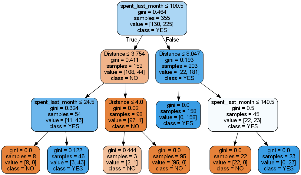
Model 4 uses the Gini impurity criterion for splitting nodes and introduces a maximum depth constraint of 3 levels, similar to Model 3 but with a different splitting criterion.
The model’s performance metrics are:
- Accuracy: 0.9832 (98.32% of predictions are correct)
- Balanced accuracy: 0.9814 (accounts for imbalanced classes)
- Precision for “Yes”: 0.9872 (98.72% of positive predictions are correct)
- Recall for “No”: 0.9756 (97.56% of actual negative cases are correctly identified)
Model 4 demonstrates excellent performance while maintaining a simple and interpretable structure. By limiting the tree depth to 3, it achieves a good balance between learning from the training data and generalizing to unseen data. The high accuracy, balanced accuracy, precision, and recall indicate that it performs well at classifying both classes without needing to be overly complex.
This model offers several advantages:
Simplicity: With a maximum depth of 3, the tree is easy to interpret and explain, which is valuable in business contexts where model interpretability is crucial. Efficiency: A shallower tree is computationally more efficient to train and use for predictions, which can be beneficial when dealing with larger datasets or when prediction speed is important. Generalization: The constrained depth helps prevent overfitting, potentially leading to better performance on new, unseen data. Feature importance: The limited depth clearly shows which features the model considers most important for classification, providing valuable insights into key factors influencing customer behavior. Balanced performance: High precision for “Yes” predictions and high recall for “No” predictions indicate that the model is reliable in identifying both positive and negative cases.
Key Observations
-
Consistency: The high performance across all models suggests that the underlying patterns in the data are strong and consistent.
-
Depth Limitation: The models with a max depth of 3 (Models 3 and 4) perform just as well as the unrestricted Gini model (Model 2). This indicates that a simple tree structure is sufficient to capture the important patterns in the data.
-
Criterion Comparison: In this case, the choice between Entropy and Gini impurity criteria doesn’t significantly impact performance when depth is limited.
-
Simplicity vs. Performance: While the unrestricted Entropy model (Model 1) shows slightly better performance, the difference is minimal. The simpler models (3 and 4) offer better interpretability without sacrificing much in terms of accuracy.
Predicting Customer Purchases
After developing our models, we can now address our primary goal: determining how many customers will buy Hidden Farm coffee. Let’s break down our findings step by step.
First, we examined the original survey data:
- In the initial survey, 303 loyal customers claimed they would purchase Hidden Farm coffee.
Next, we used our chosen model (Gini Impurity model with max depth 3) to predict potential buyers:
- The model predicted 183 additional potential buyers.
- This brings the total number of potential buyers to 486 (303 + 183).
To get a more accurate picture, we analyzed the model’s predictions on the entire surveyed population:
- Total number of surveyed people: 228
- Percentage of people predicted to buy Hidden Farm coffee: 80.26%
This result is highly promising, significantly exceeding our initial threshold of 70% for striking a deal with the local Hidden Farm farmers.
Interpretation and Decision
The model’s prediction of 80.26% potential buyers is remarkably strong, suggesting a very high interest in Hidden Farm coffee among our customer base. This percentage is well above our initial 70% threshold, which was set as the decision point for proceeding with the deal.
However, it’s crucial to note that while our model shows excellent performance, real-world factors can influence actual sales. The discrepancy between the total surveyed population (228) and the number of potential buyers (486) suggests that our model might be extrapolating beyond the initial survey data, which could introduce some uncertainty.
Despite this, the consistently high percentage of interested buyers across both the survey and the model predictions provides a strong indication of market potential.
Conclusion
Based on these results, the data strongly supports moving forward with the Hidden Farm coffee deal. The predicted interest level of 80.26% significantly exceeds our initial 70% threshold, indicating market potential for the product.
However, we must remember that data science and machine learning can inform our decisions but cannot make them for us. The final decision should consider additional factors such as:
- Risk tolerance: Are we prepared for the possibility that actual sales might not match predictions?
- Market conditions: How might external factors affect the success of Hidden Farm coffee?
- Resource allocation: Do we have the necessary resources to support this new product line?
- Long-term strategy: How does this fit into our overall business goals?
While the data provides a compelling case for proceeding with Hidden Farm coffee, the ultimate decision rests on a comprehensive evaluation of these and other relevant business factors. The strong predictive results should give us confidence, but they should be one part of a broader decision-making process.